On this page
A personal context engine is easier to trust if it can process work data locally. But local processing has a cost: time, memory, battery use, storage writes, and competition with the applications a person is already running. The phrase local-first does not tell us how expensive an implementation will be.
We measured the time required for one Python routine to build keyword postings and person-project edges from generated records. It isolates a small CPU indexing operation, separately from provider ingest, embeddings and background synchronization.
Execution environment: October 9, 2026, Python in the recorded Linux execution container. The timing samples and machine details are retained in raw.json.
Question
As the number of records grows in a fixed generated workload, how does the median time for one local Python indexing pass change? What range of measured times appears across repeats, and how much peak Python allocation is visible while tracing is enabled?
We report the process environment in the raw output so results are not mistaken for cross-device performance guarantees. Timing is especially dependent on runtime, operating system, process scheduling, and concurrent load. A single benchmark machine cannot establish user experience on other machines.
Setup
The fixture generator makes three independent collections of 250, 1,500, and 6,000 work records. Each record has a project ID, a person ID, and a body of 36 tokens sampled from a fixed vocabulary. The values are not taken from mail, calendar, Slack, source code, or personal files.
For each collection, the indexing function tokenizes the body, records each distinct token's document postings, and adds a (project, person) relationship to a set. It returns counts of unique tokens, relationship edges, and posting entries. We discard one warm-up invocation, then time seven sequential builds using perf_counter_ns. The benchmark excludes fixture generation from the timed region.
Python's tracemalloc remains enabled during the seven measured iterations and records peak traced allocation. That instrumentation adds overhead, so the numbers are not a lower bound on an optimized implementation. We chose an ordinary Python implementation precisely because its operations are easy to inspect, not because it resembles the product's production indexing pipeline.
The code produces per-trial times, a median, a minimum, a maximum, and workload counters. The output is a measurement of a real script execution, not a calculated complexity forecast.
Results
| generated records | Median build time | Range across 7 trials | Peak traced allocation |
|---|---|---|---|
| 250 | 7.0415 ms | 6.8651–7.6815 ms | 55.3 KiB |
| 1,500 | 44.2987 ms | 40.4529–49.5353 ms | 403.8 KiB |
| 6,000 | 174.8375 ms | 171.4043–214.0025 ms | 1,990.7 KiB |
The following is a textual plot of the measured medians. Each bar uses the same scale, with the longest representing the 6,000-record measurement.
  250 records | █                      7.0 ms
1,500 records | ██████                44.3 ms
6,000 records | ███████████████████████ 174.8 ms
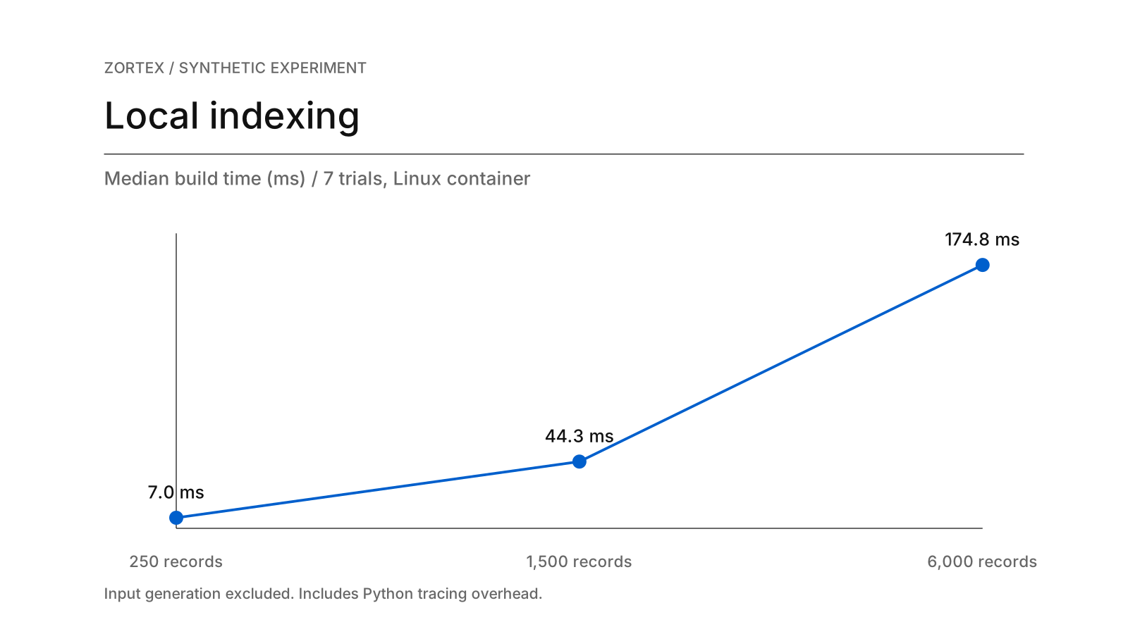
Median build times from seven instrumented passes at each generated record count.
Across these workloads, median time increases as the input grows. The observed numbers are not a proof of linear scaling; there are only three sizes, and the vocabulary is deliberately small. At 6,000 records, one of the seven trials was noticeably slower than the median. That spread is why a single headline duration would be a poor operational contract.
The peak allocation column is also easy to misinterpret. tracemalloc measures allocations traced by Python, not total resident process memory. It omits portions of native library memory, the interpreter's baseline footprint, operating-system caches, storage use, and any process that a real connector might spawn. Treat the values as debugging telemetry for this function, not estimates of how much RAM a desktop application needs.
What the measurement suggests
The first design lesson is to establish the timing boundary. Reading a mailbox over the network, parsing MIME, normalizing identities, storing encrypted records, and producing embeddings are different stages with different performance profiles. A local-first system should separately measure initial import, incremental update, query time, and background reconciliation. Combining them into one number would make regressions difficult to locate.
The second lesson is to measure work avoided. The toy function rebuilds the entire index every time. A real system should evaluate whether unchanged records can be skipped and whether small connector updates can be committed without scanning the full corpus. That may matter more to perceived performance than optimizing a tight tokenization loop.
The third is to budget for the user's machine, not merely the process's best case. A background task that looks short on an idle development container may still interrupt calls, compilation, or video playback. Useful engineering thresholds must include sustained load, energy impact, and cancellation behavior.
Measurement scope
The timed code is a Python posting-list and relationship-edge builder, separate from the desktop app and its SQLite Vault. The fixture has repetitive tokens, uniform record lengths, no binary attachments, and no cross-app parsing. It fits into memory before timing begins. The measurements were taken in a Linux container with Python; they are not macOS or Windows results.
Each input size has seven measured passes and a reported min–max range. Memory is traced allocation, not resident set size. File I/O, encryption, battery conditions, and synchronization contention are out of scope. Generated records protect private work data while making the timing input reproducible; their vocabulary and lengths are uniform.
From a full rebuild to incremental updates
Repeat this test with an incremental index, larger vocabularies, mixed document sizes, and simulated edits. Benchmark on the supported desktop operating systems, record process RSS and disk writes, and collect timing distributions while another CPU-heavy application is active. Only then set product-level budgets for initial import, per-update work, and maximum background resource use.
The exact script is experiments/local-indexing/run.py. Its raw.json contains all seven timing samples at each size, workload counters, execution-platform information, and the values plotted here. The saved timing samples make variation across reruns and runtime environments visible.